Introduction to ROOT

Overview

Teaching: min
Exercises: min

Questions

What is ROOT?

What can I learn here?

Objectives

Understand what is ROOT!

Introduction to ROOT!

What is ROOT?

Most likely some of you were already in touch with ROOT! ROOT is an open-source data analysis framework used by high energy physics and others, which lets you save and access your experiment’s data, allows you to process the data in a computationally efficient and statistically sound way and gives you access to all tools to produce publication-quality results. Basically, ROOT allows you to prcess data for physics analyses.

What can I learn here?

We would like to show you how you can perform efficient data analysis with ROOT! Starting with getting access to ROOT without any hassle, you will learn the advantages of ROOT in C++ and Python. Another ingredient for efficient analysis is a simple way to get help quickly and therefore you will learn where you can find support. ROOT can be used to go efficiently from the initial datasets to the result plots, all powered by ROOT!

Key Points

Understanding what is ROOT

Get ROOT

Overview

Teaching: min
Exercises: min

Questions

How to install ROOT on my system or get access to systems with ROOT pre-installed?

Objectives

Install ROOT

This section shows you multiple ways to get ROOT. Find below solutions to run ROOT locally, on LXPLUS, in batch systems and CIs!

Conda

Conda is a package management system and environment management system, which can install ROOT in a few minutes on Linux and MacOS.

The fastes way to get ROOT is installing Miniconda (a minimal Conda installation) and then run the following two commands:

conda create -c conda-forge --name <my-environment> root
conda activate <my-environment>

You can find detailed information about ROOT on Conda in this blog post.

CVMFS

CVMFS is a software distribution service that is already set up on many HEP systems. CMSSW including ROOT is distributed via CVMFS, but also other software stacks are available that contain ROOT.

Most notably, the CERN service LXPLUS has CVMFS always installed and enables rapid access to software and computing resources.

Docker

If you want to use ROOT in a CI system (e.g. GitLab pipelines or GitHub actions), most likely the software will be made available via Docker. The official ROOT docker containers can be found at https://hub.docker.com/r/rootproject/root. The different base images and ROOT versions are encoded in the tags, for example 6.22.00-ubuntu20.04, and latest will get you the latest ROOT release (v6.22) based on Ubuntu 20.04. If you want to try it, get Docker and run the following command to start the container with a bash shell.

docker run --rm -it rootproject/root /bin/bash

Binary releases and packages

The classic way to distribute software, besides the source code, are plain binary releases. You can download these from the release pages on https://root.cern/install/all_releases for all major MacOS and Linux versions. If you choose this installation method, make sure ROOT dependencies are installed on your system. Complete installation instructions for binary releases are available here.

In addition, for some Linux distributions, the ROOT community maintains packages in the respective package managers. You can find a list of maintained packages at https://root.cern/install/#linux-package-managers.

Verify the ROOT version

Since ROOT has a long history and numerous releases, on old systems such Scientific Linux 6 you may find correspondingly old ROOT versions. However, with the following commands you can easily verify your ROOT version and also find expert details about the ROOT configuration!

# ROOT version and build tag
root --version

# Again the ROOT version (this also works with older ROOT versions)
root-config --version

# Check that ROOT was built with C++14 support
# The output must contain one of -std=c++{14,17,1z} so that all code examples of this lesson run!
root-config --cflags

# List all the ROOT configuration options that can be checked
root-config --help

Find your way to access ROOT!

For the exercises later you need at least ROOT 6.18 and C++14 support. Feel free to set up for yourself your preferred environment satisfying this requirement!

Fallback solution

As a fallback solution you can always connect to LXPLUS via ssh -Y your_username@lxplus.cern.ch. The -Y flag enables X forwarding, which allows you to forward the output of graphics application in case you run a system with an X server such as almost all Linux distributions.

Key Points

ROOT is accessible in several different ways

Detailed up-to-date instructions can be found at https://root.cern/install

ROOT and using ROOT prompt

Overview

Teaching: min
Exercises: min

Questions

How to use a ROOT file and the ROOT prompt ?

Objectives

Open a ROOT file

Use ROOT prompt

Interactive C++

One of the main features of ROOT is the possibility to use C++ interactively thanks to the C++ interpreter Cling. Cling lets you use C++ just like Python either from the prompt or in scripts.

The ROOT prompt

By just typing root in the terminal you will enter the ROOT prompt. Like the Python prompt, the ROOT prompt is well suited to fast investigations.

$ root
root [0] 1+1
(int) 2

If you pass a file as argument to root, the file will be opened when entering the prompt and put in the variable _file0. ROOT typically comes with support for reading files remotely via HTTP (and XRootD), which we will use for the following example:

No support for remote files?

Although unlikely, your ROOT build may not be configured to support remote file access. In this case, you can just download the file with curl -O https://root.cern/files/tmva_class_example.root and point to your local file. No other changes required!

$ root tmva_class_example.root

root [0]
Attaching file mva_class_example.root as _file0...
(TFile *) 0x555f82beca10

root [1] _file0->ls() // Show content of the file, all objects are accessible via the prompt!
TWebFile**              https://root.cern/files/tmva_class_example.root
 TWebFile*              https://root.cern/files/tmva_class_example.root
  KEY: TTree    TreeS;1 TreeS
  KEY: TTree    TreeB;1 TreeB

root [2] TreeS->GetEntries() // Number of events in the dataset

root [3] TreeS->Print() // Show dataset structure
******************************************************************************
*Tree    :TreeS     : TreeS                                                  *
*Entries :     6000 : Total =           98896 bytes  File  Size =      89768 *
*        :          : Tree compression factor =   1.00                       *
******************************************************************************
*Br    0 :var1      : var1/F                                                 *
*Entries :     6000 : Total  Size=      24641 bytes  One basket in memory    *
*Baskets :        0 : Basket Size=      32000 bytes  Compression=   1.00     *
*............................................................................*
*Br    1 :var2      : var2/F                                                 *
*Entries :     6000 : Total  Size=      24641 bytes  One basket in memory    *
*Baskets :        0 : Basket Size=      32000 bytes  Compression=   1.00     *
*............................................................................*
*Br    2 :var3      : var3/F                                                 *
*Entries :     6000 : Total  Size=      24641 bytes  One basket in memory    *
*Baskets :        0 : Basket Size=      32000 bytes  Compression=   1.00     *
*............................................................................*
*Br    3 :var4      : var4/F                                                 *
*Entries :     6000 : Total  Size=      24641 bytes  One basket in memory    *
*Baskets :        0 : Basket Size=      32000 bytes  Compression=   1.00     *
*............................................................................*

root [4] TreeS->Draw("var1") // Draw a histogram of the variable var1

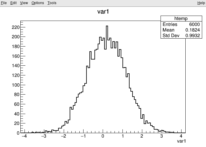
Investigating data in ROOT files

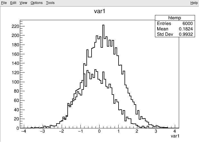
You have already seen the usage of TTree::Draw in the previous section. Such quick investigations of data in ROOT files are typical usecases which most analysts encounter on a daily basis. In the following you can learn about different ways to approach this task!

Manually plotting with `TTree::Draw`

For quick studies on the raw data in a TTree on the command line, you can use TTree::Draw to make simple visualizations:

$ root https://root.cern/files/tmva_class_example.root

root [0]
Attaching file https://root.cern/files/tmva_class_example.root as _file0...
(TFile *) 0x558d7b54aa50
root [1] TreeS->Draw("var1") // just draw var1
Info in <TCanvas::MakeDefCanvas>:  created default TCanvas with name c1
root [2] TreeS->Draw("var1", "var2 > var1", "SAME") // draw var1 with the selection var2 > var1
(long long) 3222

The `TBrowser`

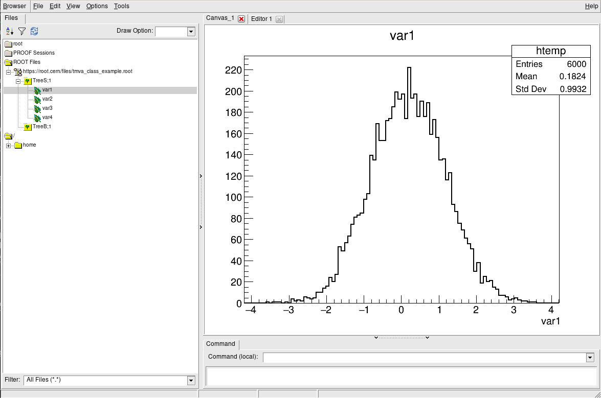
More convenient is using ROOT’s tool for browsing ROOT files, the TBrowser. You can spawn the GUI directly from the ROOT prompt as shown below.

$ root https://root.cern/files/tmva_class_example.root

root [0]
Attaching file https://root.cern/files/tmva_class_example.root as _file0...
(TFile *) 0x557892a0ef10
root [1] TBrowser b
(TBrowser &) Name: Browser Title: ROOT Object Browser

The `rootbrowse` executable

For convenience, ROOT provides the executable rootbrowse, which lets you open a TBrowser directly from the command line and display the files given as arguments!

$ rootbrowse https://root.cern/files/tmva_class_example.root

Other ROOT executables

There are many small helpers shipped with ROOT, which let you operate on data quickly from the command line and solve typical day-to-day tasks with ROOT files.

List of ROOT executables

rootbrowse: Open a ROOT file and a TBrowser
rootls: List file content, tree branches, objects’ stats
rootcp: Copy objects within a file or between files
rootdrawtree: Simple analyses from the command line
rooteventselector: Select branches, events, compression algorithms and extract slimmer trees
rootmkdir: Creates a directory in a TFile
rootmv: Move objects between files
rootprint: Print objects in plots on files
rootrm: Remove objects from files

$ rootls https://root.cern/files/tmva_class_example.root
TreeB  TreeS

$ rootls -l https://root.cern/files/tmva_class_example.root
TTree  Jan 19 14:25 2009 TreeB  "TreeB"
TTree  Jan 19 14:25 2009 TreeS  "TreeS"

$ rootls -t https://root.cern/files/tmva_class_example.root
TTree  Jan 19 14:25 2009 TreeB  "TreeB"
  var1    "var1/F"    0
  var2    "var2/F"    0
  var3    "var3/F"    0
  var4    "var4/F"    0
  weight  "weight/F"  0
  Cluster INCLUSIVE ranges:
   - # 0: [0, 5998]
   - # 1: [5999, 5999]
  The total number of clusters is 2
TTree  Jan 19 14:25 2009 TreeS  "TreeS"
  var1  "var1/F"  0
  var2  "var2/F"  0
  var3  "var3/F"  0
  var4  "var4/F"  0
  Cluster INCLUSIVE ranges:
   - # 0: [0, 5998]
   - # 1: [5999, 5999]
  The total number of clusters is 2

Try it by yourself!

Feel free to investigate the tools presented here!

Key Points

Learn hoe to open a ROOT file.

Learn to use the ROOT prompt.

ROOT scripts

Overview

Teaching: min
Exercises: min

Questions

How to use ROOT scripts?

Objectives

Learn about using C++ scripts with ROOT

This section is dedicated to the introduction to using ROOT scripts or macros.

ROOT scripts

A unique feature of ROOT is the possibility to use C++ scripts, also called “ROOT macros”. A ROOT script contains valid C++ code and uses as entrypoint a function with the same name as the script. Let’s take as example the file myScript.C with the following content.

void myScript() {
    auto file = TFile::Open("tmva_class_example.root");

    auto newtree = (TTree*)file->Get("TreeS");
    auto entries = newtree->GetEntries();
    std::cout << "Entried in TreeS : " << entries << std::endl;
}

Scripts can be processed by passing them as argument to the root executable:

$ root myScript.C

root [0]
Processing myScript.C...
Entried in TreeS  : 6000

There are other ways to run scripts, try them.

Plotting from file ith script

void myScript_plot() {

    TH1F *h_var1 = new TH1F("h_var1", "var1", 100, -4.0, 4.0);
    TFile *file = new TFile("/Users/sar/Desktop/TestROOT/tmva_class_example.root");
    TTree *tree1 = (TTree*)file->Get("TreeS");

    float var1;

    tree1->SetBranchAddress("var1", &var1);

    int nentries = (int)tree1->GetEntries();

    for(int i=0; i < nentries; i++){

        tree1->GetEntry(i);
        h_var1->Fill(var1);

    }

    TCanvas *c1 = new TCanvas();
    h_var1->Draw();
}

Examples of creating histogam:

void scriptHist(){
    auto cnt_r_h=new TH1F("count_rate",
                "Count Rate;N_{Counts};# occurencies",
                100, // Number of Bins
                -0.5, // Lower X Boundary
                15.5); // Upper X Boundary

    auto mean_count=3.6f;
    TRandom3 rndgen;
    // simulate the measurements
    for (int imeas=0;imeas<400;imeas++)
        cnt_r_h->Fill(rndgen.Poisson(mean_count));

    auto c= new TCanvas();
    cnt_r_h->Draw();

    auto c_norm= new TCanvas();
    cnt_r_h->DrawNormalized();

    // Print summary
    cout << "Moments of Distribution:\n"
         << " - Mean     = " << cnt_r_h->GetMean() << " +- "
                             << cnt_r_h->GetMeanError() << "\n"
         << " - Std Dev  = " << cnt_r_h->GetStdDev() << " +- "
                             << cnt_r_h->GetStdDevError() << "\n"
         << " - Skewness = " << cnt_r_h->GetSkewness() << "\n"
         << " - Kurtosis = " << cnt_r_h->GetKurtosis() << "\n";
}

Using graphs

// Builds a graph with errors, displays it and saves it as
// image. First, include some header files
// (not necessary for Cling)

#include "TCanvas.h"
#include "TROOT.h"
#include "TGraphErrors.h"
#include "TF1.h"
#include "TLegend.h"
#include "TArrow.h"
#include "TLatex.h"

void macro1(){
    // The values and the errors on the Y axis
    const int n_points=10;
    double x_vals[n_points]=
            {1,2,3,4,5,6,7,8,9,10};
    double y_vals[n_points]=
            {6,12,14,20,22,24,35,45,44,53};
    double y_errs[n_points]=
            {5,5,4.7,4.5,4.2,5.1,2.9,4.1,4.8,5.43};

    // Instance of the graph
    TGraphErrors graph(n_points,x_vals,y_vals,nullptr,y_errs);
    graph.SetTitle("Measurement XYZ;lenght [cm];Arb.Units");

    // Make the plot estetically better
    graph.SetMarkerStyle(kOpenCircle);
    graph.SetMarkerColor(kBlue);
    graph.SetLineColor(kBlue);

    // The canvas on which we'll draw the graph
    auto  mycanvas = new TCanvas();

    // Draw the graph !
    graph.DrawClone("APE");

    // Define a linear function
    TF1 f("Linear law","[0]+x*[1]",.5,10.5);
    // Let's make the function line nicer
    f.SetLineColor(kRed); f.SetLineStyle(2);
    // Fit it to the graph and draw it
    graph.Fit(&f);
    f.DrawClone("Same");

    // Build and Draw a legend
    TLegend leg(.1,.7,.3,.9,"Lab. Lesson 1");
    leg.SetFillColor(0);
    graph.SetFillColor(0);
    leg.AddEntry(&graph,"Exp. Points");
    leg.AddEntry(&f,"Th. Law");
    leg.DrawClone("Same");

    // Draw an arrow on the canvas
    TArrow arrow(8,8,6.2,23,0.02,"|>");
    arrow.SetLineWidth(2);
    arrow.DrawClone();

    // Add some text to the plot
    TLatex text(8.2,7.5,"#splitline{Maximum}{Deviation}");
    text.DrawClone();

    mycanvas->Print("graph_with_law.pdf");
}

int main(){
    macro1();
    }

Examples of creating a ROOT file:

void myScript_file() {

    TH1F *h_var1 = new TH1F("h_var1", "var1", 100, -4.0, 4.0);
    TFile *file = new TFile("tmva_class_example.root");
    TTree *tree1 = (TTree*)file->Get("TreeS");

    float varx;

    tree1->SetBranchAddress("var1", &varx);

    TFile* newFile( TFile::Open("newfile.root", "RECREATE") );
    auto newtree = std::make_unique<TTree>("newtree", "The Tree Title");
    newtree->Branch("branch0", &varx);

    int nentries = (int)tree1->GetEntries();

    for(int i=0; i < nentries; i++){

        tree1->GetEntry(i);
        h_var1->Fill(varx);
        newtree->Fill();

    }

    TCanvas *c1 = new TCanvas();
    h_var1->Draw();

    newFile->cd();
    newtree->Write();
    h_var1->Write();

    newFile->Write();
    newFile->Close();
}

The advantage of such scripts is the simple interaction with C++ libraries (such as ROOT) and running your code at C++ speed with the convenience of a script.

Compiled C++

You can improve the runtime of your programs if you compile them upfront. Therefore, ROOT tries to make the compilation of ROOT macros as convenient as possible!

ACLiC

ROOT provides a mechanism called ACLiC to compile the script in a shared library and call the compiled code from interactive C++, all automatically!

The only change required to our script is that we need to include all required headers:

#include "TFile.h"
#include "TTree.h"
#include <iostream>

void myScript() {
    // The body of the myScript function goes here
}

Now, let’s compile and run the script again. Note the + after the script name!

$ root myScript.C+

ACLiC has many more features, for example compiling your program with debug symbols using +g. You can find the documentation here.

C++ compilers

Of course, the C++ code can also just be compiled with C++ compilers such as g++ or clang++ with the advantage that you have full control of all compiler settings, most notable the optimization flags such as -O3!

To do so, we have to add the main function to the script, which is the default entrypoint for C(++) programs.

#include "TFile.h"
#include "TTree.h"
#include <iostream>

void myScript() {
    // The body of the myScript function goes here
}

int main() {
    myScript();
    return 0;
}

Now, you can use the following command with your C++ compiler of choice to compile the script into an executable.

$ g++ -O3 -o myScript myScript.C $(root-config --cflags --libs)
$ ./myScript
TreeS : 6000
TreeB : 6000

Computationally heavy programs and long running analyses may benefit greatly from the optimized compilation with -O3 and can save you hours of computing time!

Key Points

ROOT provides many features from histogramming, fitting and plotting to investigating data interactively in C++ and Python but scripts can help with advanced work

Learn about C/C++ scripts for ROOT.

Using ROOT with Python

Overview

Teaching: min
Exercises: min

Questions

How can I use ROOT with Python?

Objectives

Learn about the basics of ROOT with Python

Python

ROOT provides the Python bindings called PyROOT. PyROOT is not just ROOT from Python, but a full-featured interface to call C++ libraries in a pythonic way. This lets you import the ROOT module from Python and makes all features dynamically available. Let’s rewrite the C++ example from above and put the code in the file myScript.py!

import ROOT

rfile = ROOT.TFile.Open('https://root.cern/files/tmva_class_example.root')
for key in rfile.GetListOfKeys():
    name = key.GetName()
    entries = rfile.Get(name).GetEntries()
    print('{} : {}'.format(name, entries))

Calling the Python script works as expected:

$ python myScript.py
TreeS : 6000
TreeB : 6000

But PyROOT can do much more for you than simply providing access to C++ libraries from Python. You can also inject efficient C++ code into your Python program to speed up potentially slow parts of your program!

import ROOT

ROOT.gInterpreter.Declare('''
int my_heavy_computation(std::string x) {
    // heavy computation goes here
    return x.length();
}
''')

# Functions and object made available via the interpreter are accessible from
# the ROOT module
y = ROOT.my_heavy_computation("the ultimate answer to life and everything")
print(y) # Guess the result!

Basic histogramming, fitting and plotting

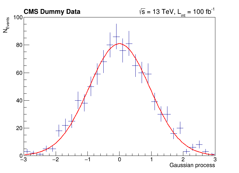
The following script uses basic features from ROOT, which are used commonly in day-to-day work with ROOT. You can investigate the typical workflow to create histograms with TH1F, fit a function to the data with TF1 and produce an accurate visualization with TCanvas and others. Below, you can see the output of the fit to the data with the measured parameters.

import ROOT
import numpy as np

# Make global style changes
ROOT.gStyle.SetOptStat(0) # Disable the statistics box
ROOT.gStyle.SetTextFont(42)

# Create a canvas
c = ROOT.TCanvas('c', 'my canvas', 800, 600)

# Create a histogram with some dummy data and draw it
data = np.random.randn(1000).astype(np.float32)
h = ROOT.TH1F('h', ';Gaussian process; N_{Events}', 30, -3, 3)
for x in data: h.Fill(x)
h.Draw('E')

# Fit a Gaussian function to the data
f = ROOT.TF1('f', '[0] * exp(-0.5 * ((x - [1]) / [2])**2)')
f.SetParameters(100, 0, 1)
h.Fit(f)

# Let's add some CMS style headline
label = ROOT.TLatex()
label.SetNDC(True)
label.SetTextSize(0.040)
label.DrawLatex(0.10, 0.92, '#bf{CMS Dummy Data}')
label.DrawLatex(0.58, 0.92, '#sqrt{s} = 13 TeV, L_{int} = 100 fb^{-1}')

# Save as png file and show interactively
c.SaveAs('dummy_data.png')
c.Draw()

 FCN=30.2937 FROM MIGRAD    STATUS=CONVERGED      67 CALLS          68 TOTAL
                     EDM=1.34686e-08    STRATEGY= 1      ERROR MATRIX ACCURATE
  EXT PARAMETER                                   STEP         FIRST
  NO.   NAME      VALUE            ERROR          SIZE      DERIVATIVE
   1  p0           8.09397e+01   3.19887e+00   7.10307e-03  -3.40988e-05
   2  p1          -3.46483e-03   3.10501e-02   8.47265e-05  -2.30742e-03
   3  p2           9.56532e-01   2.24141e-02   4.97399e-05   2.58872e-03
Info in <TCanvas::Print>: file dummy_data.png has been created

Try it by yourself!

Run the example code by yourself! In case the execution ends without displaying the plot on screen, you can run the script in interpreted mode with python -i your_script.py. That will keep the process alive after the plot is displayed.

A guide to such advanced features of PyROOT can be found in the official manual at https://root.cern/manual/python. Feel free to investigate!

Interoperability with NumPy arrays

There are many reasons, for example machine learning applications, to want to export your data in Python to NumPy arrays. This is easily possible with ROOT and is part of RDataFrame. The code snippets below show you how to do this conversion and how to move the data to typical tools in the Python ecosystem, e.g., numpy and pandas.

numpy and pandas

Have you installed numpy and pandas or are you on a system which has them available? Normally, you can just run pip install --user numpy pandas to install missing packages! Another option is searching in your system package manager, they are typically available on all platforms.

Convert data in ROOT files to numpy arrays

The conversion feature is attached to the class RDataFrame. We will not introduce you here to this way to process data with ROOT because the following section is dedicated to RDataFrame. For now, just keep in mind that you call AsNumpy! The data is returned as a dictionary of one-dimensional numpy arrays.

# Read out the data as a dictionary of numpy arrays
import ROOT
df = ROOT.RDataFrame('TreeS', 'https://root.cern/files/tmva_class_example.root')
columns = ['var1', 'var2', 'var3', 'var4']
data = df.AsNumpy(columns)
print('var1: {}'.format(data['var1']))

var1: [-1.1436108   2.1434433  -0.44391322 ...  0.37746507 -2.072639 -0.09141494]

Move the data to numpy or pandas

The data can be passed naturally to any method in the Python ecosystem which processes numpy arrays. Below is an example that computes the mean of each column.

# Apply numpy methods
import numpy as np
print('Means: {}'.format([np.mean(data[c]).item() for c in columns]))

Means: [0.18244409561157227, 0.28425973653793335, 0.3789360225200653, 0.7712161540985107]

Another interesting usecase is moving the dataset directly to a pandas dataframe. You can use the output of AsNumpy directly as input to its constructor.

# Convert to a pandas dataframe
import pandas
pdf = pandas.DataFrame(data)
print(pdf)

          var1      var2      var3      var4
  -1.143611 -0.822373 -0.495426 -0.629427
   2.143443 -0.018923  0.267030  1.267493
  -0.443913  0.486827  0.139535  0.611483
   0.281100 -0.347094 -0.240525  0.347208
   0.604006  0.151232  0.964091  1.227711
...        ...       ...       ...       ...
-0.040650 -0.154212 -0.097715  0.440331
0.099931 -1.183759  0.034616  0.644502
0.377465 -0.030945  1.166082  0.728614
-2.072639 -0.635586 -0.747371 -1.285679
-0.091415  0.221271  0.569032  1.386130

[6000 rows x 4 columns]

Try it by yourself!

The statements are very short, you can just copy paste them into the Python prompt. Feel free to investigate what you can do with AsNumpy! Further information can be found here.

ROOT in Jupyter notebooks

ROOT provides a deep integration with Jupyter notebooks. You can start a Jupyter notebook server including ROOT features with the following command:

root --notebook

Alternatively, you can go to https://swan.cern.ch, which provides Jupyter notebooks integrated with CERN’s cloud storage as a web service. Note that you may have to visit https://cernbox.cern.ch first at least once with your user account to create your CERNBox space!

Python kernel

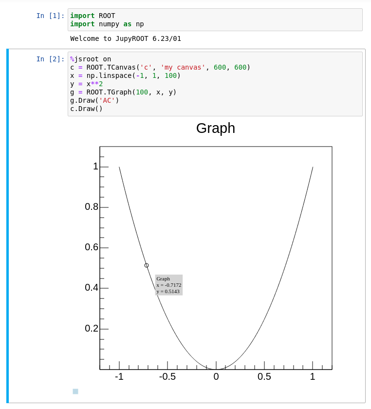
Jupyter is often use to edit Python code interactively. By creating a new notebook with a Python kernel, you will see something similar to the screenshot below and you can work interactively with Python in the browser!

C++ kernel

ROOT provides a Jupyter C++ kernel, which behaves similarly to the Python kernel but for C++! Similar to the ROOT prompt, you can work interactively with C++ in the notebook. Just select the C++ kernel in the drop-down menu!

JSROOT

Another feature of ROOT is the %jsroot on magic, which enables ROOT’s JavaScript integration! This allows you to interact with the visualization such as you are used to it from the interactive graphics in the Python prompt.

Because it’s JavaScript, we can also embed these plots easily in any website. You can find an interactive version of the plot from the top of this section at the bottom of the page. For example, you can zoom in, add grid lines or get detailed information about the data points, right here!

Try it by yourself!

Either run Jupyter locally via root --notebook or go to https://swan.cern.ch to try ROOT in a Jupyter notebook!

More useful features

ROOT is made for HEP analysis and contains many other features that are useful in typical tasks, for example:

TEfficiency, to handle histograms representing efficiencies and their uncertainties
THStack, to stack histograms
TRatioPlot, to create ratio plots with the histograms on the top and the ratio with the correct uncertainties on the bottom
And many more!

Try using ROOT with interactive C++, compiled C++ and Python!

Make yourself familiar with the different ways you can run an analysis with ROOT!

Key Points

ROOT can be used with python

PyROOT lets you use C++ from Python but offers many more advanced features to speed up your analysis in Python. Details about the dynamic Python bindings provided by PyROOT can be found on https://root.cern/manual/python.

How to get help with ROOT?

Overview

Teaching: min
Exercises: min

Questions

Where can I find documentation?

Where can I ask for help?

Objectives

Learn how to find the official documentation!

Learn about the ROOT forum to get help!

Something does not work as expected, how can I get help?

User support is an integral part of ROOT and happily provided by the ROOT team!

We provide multiple communication channels so that we can help you but also you can help yourself to find the right answers to your questions, as fast as possible!

Support and discussion channel for this lesson

Communication channels for support and discussion dedicated to this lesson are linked on the front page!

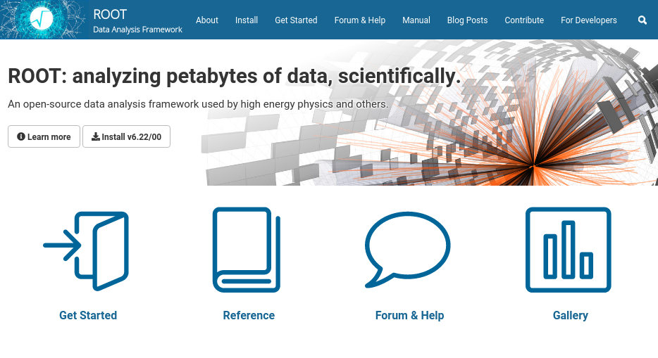
The ROOT website, the beginner’s guide and the manual

The ROOT website is home to the beginner’s guide and the more in-depth manual. These are a great resource to start with ROOT and learn about parts of the framework in high detail. Keep in mind the ROOT website at https://root.cern, which provides links to all resources in a single place!

The reference guide

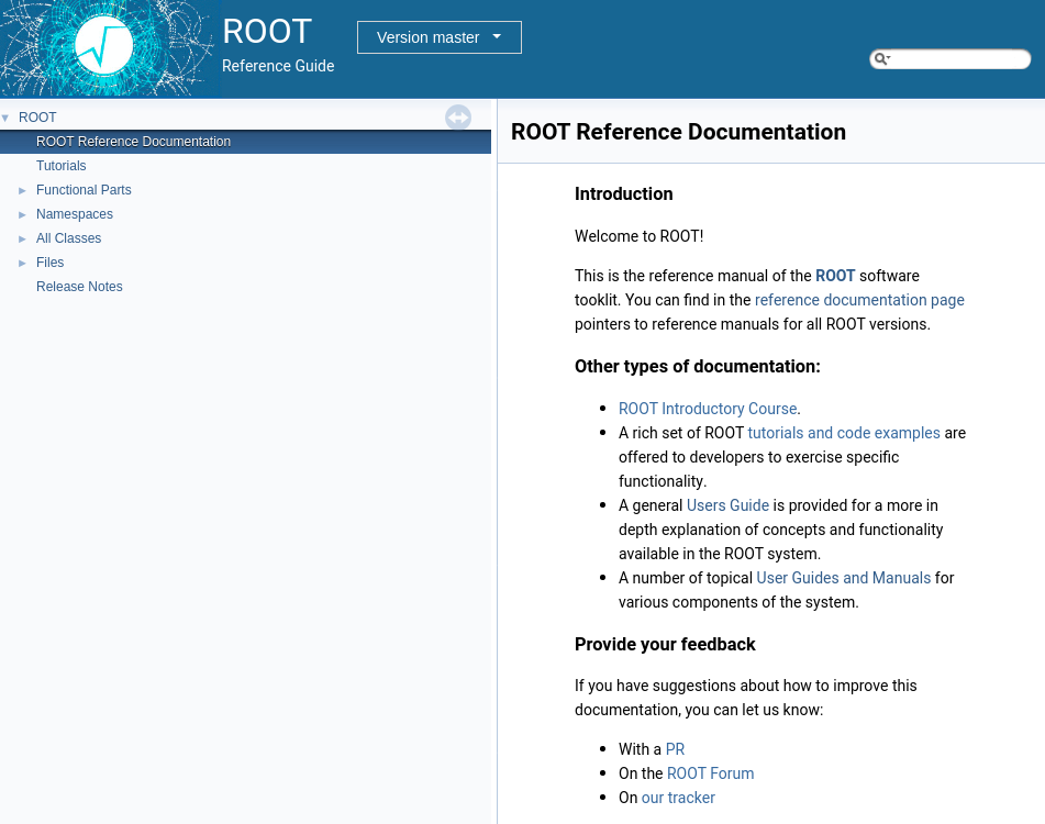
The reference guide provides a more technical documentation about ROOT powered by Doxygen. You can search for classes or functions in ROOT, learn about types and methods and trace features down to the actual implementation.

Although the reference guide is more technical in first place, important classes have extensive additional documentation. Feel free to investigate TTree or RDataFrame!

Another part of the reference guide are the tutorials, which explain features in working code examples. Feel free to look at tutorials for RooFit and RDataFrame, which cover many typical use cases for these parts of ROOT!

The ROOT forum

The ROOT forum is the to-go place if you cannot find the answer in the documentation. Don’t hesitate to open a discussion, there is always someone from the ROOT team actively taking care of new questions in the forum!

But not only questions are very welcome, you can also discuss possible improvements or make suggestions for new features!

Bug tracking

Bugs are currently tracked on Jira, but we will soon switch to GitHub issues. However, if you discover bugs, please report them! In case you are not sure whether you see a bug or a feature, posting in the ROOT forum is always a good idea and always appreciated!

Key Points

User support is an integral part of ROOT!

https://root.cern is the entry point to find all documentation

The reference guide provides in-depth technical documentation, but also additional explanation for classes and a huge amount of tutorials explaining features with code

The ROOT forum is actively maintained by the ROOT team to support you!

Assignment 1 Hints

Overview

Teaching: min
Exercises: min

Questions

How to complete Assignment 1 ?

Objectives

Complete Assignment 1

Read and write file with arrays as branches and calculating invariant mass

The following script should help you understand how to read and write a file with arrays as branches, and some hints on calculating invariant mass of a particle that decays to two objects which are reconstructed. Do read the comments embedded within the code.

void myScript() {
    auto inputfile = TFile::Open("DYJetsToLL.root");

    auto inputtree = (TTree*)inputfile->Get("Events");
    long nentries = inputtree->GetEntries();

    const int nmuonmax = 50;// a number higher than maximum number of muons in any event in the file
    const int ntaumax = 50;// a number higher than maximum number of taus in any event in the file
    
    uint nmuon;
    uint ntau;
    float taupt[ntaumax];//these are arrays, that is they contain multiple numbers
    float tauphi[ntaumax];
    float taueta[ntaumax];
    float taumass[ntaumax];
    int taucharge[ntaumax];
    bool tauisotight[ntaumax]; //this is a boolean array

    TLorentzVector lvectau1, lvectau2, lvecZ;//Lorentz vectors
    float ditaumass;
    
    //Setting branches of input file and tree to the variables

    inputtree->SetBranchAddress("nMuon", &nmuon);
    inputtree->SetBranchAddress("nTau", &ntau);
    inputtree->SetBranchAddress("Tau_pt", taupt); //syntax for assigning branches to arrays
    inputtree->SetBranchAddress("Tau_phi", tauphi);
    inputtree->SetBranchAddress("Tau_eta", taueta);
    inputtree->SetBranchAddress("Tau_charge", taucharge);
    inputtree->SetBranchAddress("Tau_mass", taumass);
    inputtree->SetBranchAddress("Tau_idIsoTight", tauisotight); //this is a boolean array
    
    //Output file
  
    TFile* newFile( TFile::Open("newfile.root", "RECREATE") );
    auto newtree = std::make_unique<TTree>("newtree", "Events");
    newtree->Branch("nTau", &ntau, "nTau/I");//no need for the "nTau/I" as it takes it as default, but specifying for following cases
    newtree->Branch("Tau_pt", taupt, "Tau_pt[nTau]/F");//for arrays, need to specify in the third argument that it is an array (notice, no & sign in second arguments for array) of size ntau and store float variable


    //Output histograms
    auto hntau = new TH1F("hntau", "Number of Taus", 50, -0.5, 49.5);
    auto htaupt = new TH1F("htaupt", "Tau pT", 100, 0.0, 200.0);
    
    //Event loop
     std::cout<<"Entering event loop"<<std::endl;

    for (int i = 0; i < int(nentries); i++){
        inputtree->GetEntry(i);
        hntau->Fill(ntau);
        for (auto j = 0; j < ntau; j++){
            htaupt->Fill(taupt[j]);
        }
        if (ntau >= 2){
            lvectau1.SetPtEtaPhiM(taupt[0],taueta[0],tauphi[0],taumass[0]); //leading taus are the first two, that is with index 0,1
            lvectau2.SetPtEtaPhiM(taupt[1],taueta[1],tauphi[1],taumass[1]);
            lvecZ = lvectau1+lvectau2;
            ditaumass = lvecZ.Mag(); // invariant mass
        }
        newtree->Fill();

    }

    std::cout<<"End of event loop"<<std::endl;

    inputfile->Close();
    
    //Writing output file
    newFile->cd();
    newFile->Write();
    newFile->Close();
    newFile->Delete();
    std::cout<<"End of script"<<std::endl;
}

Key Points

Some help with Assignment 1

Get DELPHES

Overview

Teaching: min
Exercises: min

Questions

What is DELPHES ?

How to install DELPHES ?

Objectives

Install DELPHES

DELPHES

Delphes framework for fast detector response simulation. The simulation includes a tracking system, embedded into a magnetic field, calorimeters and a muon system. The framework is interfaced to standard file formats (e.g. Les Houches Event File or HepMC) and outputs observables such as isolated leptons, missing transverse energy and collection of jets which can be used for dedicated analyses. The simulation of the detector response takes into account the effect of magnetic field, the granularity of the calorimeters and sub-detector resolutions. Visualisation of the final state particles is also built-in using the corresponding ROOT library.

DELPHES documentation

The official webpage for DELPHES can be found here. The publication detailing DELPHES can be found at JHEP 02 (2014) 057 or arXiv:1307.6346.

Installing DELPHES

To successfully install Delphes the following prerequisite packages should be installed: ROOT and Tcl scripting language.

Download and build Delphes after sourcing ROOT:

$ wget http://cp3.irmp.ucl.ac.be/downloads/Delphes-3.5.0.tar.gz
$ tar -zxf Delphes-3.5.0.tar.gz
$ cd Delphes-3.5.0
$ make

Key Points

The official webpage for DELPHES can be found here

Introduction to DELPHES

Overview

Teaching: min
Exercises: min

Questions

What is DELPHES ?

How to use DELPHES ?

Objectives

Working with DELPHES

DELPHES

DELPHES documentation

The official webpage for DELPHES can be found here. The publication detailing DELPHES can be found at JHEP 02 (2014) 057 or arXiv:1307.6346.

Running DELPHES

Running Delphes can be done through the executables in the directory while passing arguments and paramteres. Eg.:

./DelphesHepMC3

But with parameters. When running Delphes without parameters or when supplying an invalid command line, the following message will be shown:

 Usage: DelphesHepMC3 config_file output_file [input_file(s)]
 config_file - configuration file in Tcl format,
 output_file - output file in ROOT format,
 input_file(s) - input file(s) in HepMC format,
 with no input_file, or when input_file is -, read standard input.

Running Delphes with HepMC input files (example):

./DelphesHepMC3 cards/delphes_card_CMS.tcl output.root input.hepmc

Try using with the file ttbar.lhe shared with you.

./DelphesLHEF cards/delphes_card_CMS.tcl delphes_output.root ttbar.lhe

DELPHES produced output ROOT file

To understand the content of the ROOT file produced, a handy reference is available at the Delphes webpage linked here.

To open the file with ROOT, you need to first load the Delphes library with which the contents of the file can be read:

$ root 
root[0] gSystem->Load("libDelphes");

Then you can open the Delhes output ROOT file as:

$ root 
root[0] gSystem->Load("libDelphes");
root[1] TFile *_file0 = TFile::Open("delphes_output.root")
root[3] TBrowser browser

Visualising DELPHES Detector Simulation

Delphes also allows to viualise event by event detector simulation. Try it out:

$ make display
$ root -l examples/EventDisplay.C'("cards/delphes_card_CMS.tcl","delphes_output.root")'

Running DELPHES directly with PYTHIA8

For this, you need a working PYTHIA8 installation (assuming you have that from the first part of the course).

Define an environment variable for the path to your PYTHIA installation directory:

$ export PYTHIA8=path_to_PYTHIA8_installation 
$ echo $PYTHIA8

Then, in your DELPHES directory, build the “DelphesPythia8” executable with the following command:

$ make HAS_PYTHIA8=true

Now, you can run a simple example for generating Pythia8 events within Delphes:

$ ./DelphesPythia8 cards/delphes_card_CMS.tcl examples/Pythia8/configNoLHE.cmnd delphes_pythia8.root

Key Points

Understanding basics of using DELPHES.

The publication detailing DELPHES can be found at JHEP 02 (2014) 057 or arXiv:1307.6346

DELPHES with Scripts

Overview

Teaching: min
Exercises: min

Questions

How to analyse DELPHES output files with scripts for ROOT?

Objectives

Learning about using DELPHES with C and Python scripts

DELPHES with basic scripts

Try to save the following script as file “DelphesScript1.C” and then run it as:

root
gSystem->Load("libDelphes");
.x DelphesScript1.C("delphes_output.root");

The script:

void DelphesScript1(const char *inputFile)
{
  gSystem->Load("libDelphes");

  // Create chain of root trees
  TChain chain("Delphes");
  chain.Add(inputFile);
  
  // Create object of class ExRootTreeReader
  ExRootTreeReader *treeReader = new ExRootTreeReader(&chain);
  Long64_t numberOfEntries = treeReader->GetEntries();
  
  // Get pointers to branches used in this analysis
  TClonesArray *branchJet = treeReader->UseBranch("Jet");
  TClonesArray *branchElectron = treeReader->UseBranch("Electron");
  
  // Book histograms
  TH1 *histJetPT = new TH1F("jet_pt", "jet P_{T}", 100, 0.0, 100.0);
  TH1 *histMass = new TH1F("mass", "M_{inv}(e_{1}, e_{2})", 100, 40.0, 140.0);

  // Loop over all events
  for(Int_t entry = 0; entry < numberOfEntries; ++entry)
  {
    // Load selected branches with data from specified event
    treeReader->ReadEntry(entry);
  
    // If event contains at least 1 jet
    if(branchJet->GetEntries() > 0)
    {
      // Take first jet
      Jet *jet = (Jet*) branchJet->At(0);
      
      // Plot jet transverse momentum
      histJetPT->Fill(jet->PT);
      
      // Print jet transverse momentum
      cout << jet->PT << endl;
    }

    Electron *elec1, *elec2;

    // If event contains at least 2 electrons
    if(branchElectron->GetEntries() > 1)
    {
      // Take first two electrons
      elec1 = (Electron *) branchElectron->At(0);
      elec2 = (Electron *) branchElectron->At(1);

      // Plot their invariant mass
      histMass->Fill(((elec1->P4()) + (elec2->P4())).M());
    }
  }

  // Show resulting histograms
  histJetPT->Draw();
}

DELPHES with more advanced scripts

The following script can be run as:

root DelphesScript2.C'("delphes_output.root")'

The scripts “DelphesScript2.C” :

#include "TH1.h"
#include "TSystem.h"

#ifdef __CLING__
R__LOAD_LIBRARY(libDelphes)
#include "classes/DelphesClasses.h"
#include "external/ExRootAnalysis/ExRootTreeReader.h"
#include "external/ExRootAnalysis/ExRootResult.h"
#endif

//------------------------------------------------------------------------------

struct MyPlots
{
  TH1 *fJetPT[2];
  TH1 *fMissingET;
  TH1 *fElectronPT;
};

//------------------------------------------------------------------------------

class ExRootResult;
class ExRootTreeReader;

//------------------------------------------------------------------------------

void BookHistograms(ExRootResult *result, MyPlots *plots)
{
  THStack *stack;
  TLegend *legend;
  TPaveText *comment;

  // book 2 histograms for PT of 1st and 2nd leading jets

  plots->fJetPT[0] = result->AddHist1D(
    "jet_pt_0", "leading jet P_{T}",
    "jet P_{T}, GeV/c", "number of jets",
    50, 0.0, 100.0);

  plots->fJetPT[1] = result->AddHist1D(
    "jet_pt_1", "2nd leading jet P_{T}",
    "jet P_{T}, GeV/c", "number of jets",
    50, 0.0, 100.0);

  plots->fJetPT[0]->SetLineColor(kRed);
  plots->fJetPT[1]->SetLineColor(kBlue);

  // book 1 stack of 2 histograms

  stack = result->AddHistStack("jet_pt_all", "1st and 2nd jets P_{T}");
  stack->Add(plots->fJetPT[0]);
  stack->Add(plots->fJetPT[1]);

  // book legend for stack of 2 histograms

  legend = result->AddLegend(0.72, 0.86, 0.98, 0.98);
  legend->AddEntry(plots->fJetPT[0], "leading jet", "l");
  legend->AddEntry(plots->fJetPT[1], "second jet", "l");

  // attach legend to stack (legend will be printed over stack in .eps file)

  result->Attach(stack, legend);

  // book more histograms

  plots->fElectronPT = result->AddHist1D(
    "electron_pt", "electron P_{T}",
    "electron P_{T}, GeV/c", "number of electrons",
    50, 0.0, 100.0);

  plots->fMissingET = result->AddHist1D(
    "missing_et", "Missing E_{T}",
    "Missing E_{T}, GeV", "number of events",
    60, 0.0, 30.0);

  // book general comment

  comment = result->AddComment(0.64, 0.86, 0.98, 0.98);
  comment->AddText("demonstration plot");
  comment->AddText("produced by Example2.C");

  // attach comment to single histograms

  result->Attach(plots->fJetPT[0], comment);
  result->Attach(plots->fJetPT[1], comment);
  result->Attach(plots->fElectronPT, comment);

  // show histogram statisics for MissingET
  plots->fMissingET->SetStats();
}

//------------------------------------------------------------------------------

void AnalyseEvents(ExRootTreeReader *treeReader, MyPlots *plots)
{
  TClonesArray *branchJet = treeReader->UseBranch("Jet");
  TClonesArray *branchElectron = treeReader->UseBranch("Electron");
  TClonesArray *branchMissingET = treeReader->UseBranch("MissingET");

  Long64_t allEntries = treeReader->GetEntries();

  cout << "** Chain contains " << allEntries << " events" << endl;

  Jet *jet[2];
  MissingET *met;
  Electron *electron;

  Long64_t entry;

  Int_t i;

  // Loop over all events
  for(entry = 0; entry < allEntries; ++entry)
  {
    // Load selected branches with data from specified event
    treeReader->ReadEntry(entry);

    // Analyse two leading jets
    if(branchJet->GetEntriesFast() >= 2)
    {
      jet[0] = (Jet*) branchJet->At(0);
      jet[1] = (Jet*) branchJet->At(1);

      plots->fJetPT[0]->Fill(jet[0]->PT);
      plots->fJetPT[1]->Fill(jet[1]->PT);
    }

    // Analyse missing ET
    if(branchMissingET->GetEntriesFast() > 0)
    {
      met = (MissingET*) branchMissingET->At(0);
      plots->fMissingET->Fill(met->MET);
    }

    // Loop over all electrons in event
    for(i = 0; i < branchElectron->GetEntriesFast(); ++i)
    {
      electron = (Electron*) branchElectron->At(i);
      plots->fElectronPT->Fill(electron->PT);
    }
  }
}

//------------------------------------------------------------------------------

void PrintHistograms(ExRootResult *result, MyPlots *plots)
{
  result->Print("png");
}

//------------------------------------------------------------------------------

void DelphesScript2(const char *inputFile)
{
  gSystem->Load("libDelphes");

  TChain *chain = new TChain("Delphes");
  chain->Add(inputFile);

  ExRootTreeReader *treeReader = new ExRootTreeReader(chain);
  ExRootResult *result = new ExRootResult();

  MyPlots *plots = new MyPlots;

  BookHistograms(result, plots);

  AnalyseEvents(treeReader, plots);

  PrintHistograms(result, plots);

  result->Write("results.root");

  cout << "** Exiting..." << endl;

  delete plots;
  delete result;
  delete treeReader;
  delete chain;
}

DELPHES with python scripts

The following script can be run as:

python DelphesPythonScript.py delphes_output.root

The script “DelphesPythonScript.py” :

#!/usr/bin/env python

import sys

import ROOT

try:
  input = raw_input
except:
  pass

if len(sys.argv) < 2:
  print(" Usage: Example1.py input_file")
  sys.exit(1)

ROOT.gSystem.Load("libDelphes")

try:
  ROOT.gInterpreter.Declare('#include "classes/DelphesClasses.h"')
  ROOT.gInterpreter.Declare('#include "external/ExRootAnalysis/ExRootTreeReader.h"')
except:
  pass

inputFile = sys.argv[1]

# Create chain of root trees
chain = ROOT.TChain("Delphes")
chain.Add(inputFile)

# Create object of class ExRootTreeReader
treeReader = ROOT.ExRootTreeReader(chain)
numberOfEntries = treeReader.GetEntries()

# Get pointers to branches used in this analysis
branchJet = treeReader.UseBranch("Jet")
branchElectron = treeReader.UseBranch("Electron")

# Book histograms
histJetPT = ROOT.TH1F("jet_pt", "jet P_{T}", 100, 0.0, 100.0)
histMass = ROOT.TH1F("mass", "M_{inv}(e_{1}, e_{2})", 100, 40.0, 140.0)

# Loop over all events
for entry in range(0, numberOfEntries):
  # Load selected branches with data from specified event
  treeReader.ReadEntry(entry)

  # If event contains at least 1 jet
  if branchJet.GetEntries() > 0:
    # Take first jet
    jet = branchJet.At(0)

    # Plot jet transverse momentum
    histJetPT.Fill(jet.PT)

    # Print jet transverse momentum
    print(jet.PT)

  # If event contains at least 2 electrons
  if branchElectron.GetEntries() > 1:
    # Take first two electrons
    elec1 = branchElectron.At(0)
    elec2 = branchElectron.At(1)

    # Plot their invariant mass
    histMass.Fill(((elec1.P4()) + (elec2.P4())).M())

# Show resulting histograms
histJetPT.Draw()

input("Press Enter to continue...")

More complex Python code can be written based on a separate analysis package, deteailed at DelphesAnalysis.

Key Points

Learning about using DELPHES with C and Python scripts

More complex Python code can be written based on a separate analysis package, deteailed at DelphesAnalysis.

Computational Particle Physics Course

Introduction to ROOT

Overview

What is ROOT?

What can I learn here?

Key Points

Get ROOT

Overview

Conda

CVMFS

Docker

Binary releases and packages

Verify the ROOT version

Find your way to access ROOT!

Fallback solution

Key Points

ROOT and using ROOT prompt

Overview

Interactive C++

The ROOT prompt

No support for remote files?

Investigating data in ROOT files

Manually plotting with TTree::Draw

The TBrowser

The rootbrowse executable

Other ROOT executables

Try it by yourself!

Key Points

ROOT scripts

Overview

ROOT scripts

Plotting from file ith script

Examples of creating histogam:

Using graphs

Examples of creating a ROOT file:

Compiled C++

ACLiC

C++ compilers

Key Points

Using ROOT with Python

Overview

Python

Basic histogramming, fitting and plotting

Try it by yourself!

Interoperability with NumPy arrays

numpy and pandas

Convert data in ROOT files to numpy arrays

Move the data to numpy or pandas

Try it by yourself!

ROOT in Jupyter notebooks

Python kernel

C++ kernel

JSROOT

Try it by yourself!

More useful features

Try using ROOT with interactive C++, compiled C++ and Python!

Key Points

How to get help with ROOT?

Overview

Something does not work as expected, how can I get help?

Support and discussion channel for this lesson

The ROOT website, the beginner’s guide and the manual

The reference guide

The ROOT forum

Bug tracking

Key Points

Assignment 1 Hints

Overview

Read and write file with arrays as branches and calculating invariant mass

Key Points

Get DELPHES

Overview

DELPHES

DELPHES documentation

Installing DELPHES

Key Points

Introduction to DELPHES

Overview

DELPHES

DELPHES documentation

Manually plotting with `TTree::Draw`

The `TBrowser`

The `rootbrowse` executable